
Working with named cells in Excel via Visual Cash Focus
Excel and named cells
Named cells is a feature of Excel.
- A name (e.g. TOTAL) can be used instead of a normal cell reference (A1).
- Names must be unique within the spreadsheet.
Excel interface to Visual Cash Focus
Using Excel is optional! One can type the numbers directly into the table on the Budget per period page. However, sometimes it can be useful to use Excel to do calculations and import the results into the table.
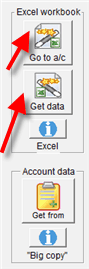
On the Budget per period page there are two buttons to link the budget to an Excel spreadsheet:-
Go to a/c (account) button: This opens Excel and positions you on the current account number (if it exists in Excel). If it does not exist, it will be created (assuming that the default properties are set correctly – discussed below).
Get data button: This transfers data from Excel into Visual Cash Focus for the account number being viewed. If the Excel spreadsheet has data for this account number, then it will be transferred into the Budget per period table and will be seen directly.
Note: The Excel spreadsheet is a supporting document. When the Excel data is imported into the table, it will be used by the software.
How does Visual Cash Focus link to Excel? The account number is the link between the software and Excel. Named cells are used to locate account numbers in a spreadsheet. The link to Excel is via the account number with a prefix of “_”.
Example:
Account number: HATS
Named cell in Excel: _HATS.
(Notice the underscore in front of HATS).
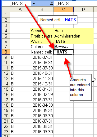
Notice in the picture above that the cell name is shown on the top left – just above the A column.
When you click in a cell, it will either show the cell reference (C8) or the cell name (_HATS) if the cell has been named.
Tip: The link is automatic and you should not usually need to worry about the above – the software will do it all for you. A named cell will be created automatically in Excel. (Try it and see how easily it works!)
Note: To comply with Excel naming conventions, any spaces in the account number are changed automatically to “.” and funny characters like # are changed to “_”. If you need it, you can see the name of the cell for any account by click the Excel “i” button.
Another example:
The account number: “BLOOD TESTS” corresponds to the named cell: “_BLOOD.TESTS”.
Named cell magic
In Visual Cash Focus, when you go to the account, a named cell will be created automatically at the bottom of the spreadsheet.
Note: When Visual Cash Focus imports data from Excel, it looks for a named cell, and then the column directly underneath the named cell. It will import whatever data it finds there. When you first Go to the account, if it doesn’t exist yet, the software adds additional information above and to the left of the named cell. This information is for the convenience of the user, and is not read by the software. it should be regarded as decoration only, as far as the software is concerned. Sometimes the second column will be used, if appropriate. For example, if revenue is budgeted as price per quantity, the column directly under the named cell will be price, the column directly adjacent will be price. If you let the software create the named cell for you, the “decoration” that gets added to the Excel spreadsheet will identify the columns for you.
Note: The software always adds a new account underneath the last occupied row. It has no ability to add a named cell next to the previous one. But you can move it to wherever you want, even to another sheet in the same spreadsheet.
Cut and paste
Select the appropriate cells in Excel, including the named cell. Then “Cut and Paste” to a new location. The named cell will move to the new location. You can see that by clicking on the named cell and looking at the cell reference, which is shown at the top above the A column.
How to delete a named cell
Sometimes you may want to delete a named cell. Excel provides this functionality.
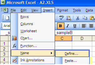
In Excel versions prior to Excel 2007, go to the Insert menu. Choose Name, then Define.
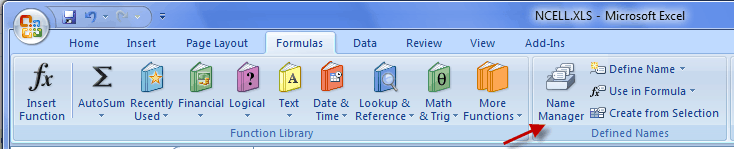
In Excel versions from Excel 2007: open the Name Manager dialog box as follows:-
On the Formulas tab, in the Defined Names group, click Name Manager.
You see a list of the named cells – click on the appropriate one and click Delete and remove it.
In Excel versions from Excel 2007, more information is available in the Excel help file, under: Manage names by using the Name Manager dialog box.
How to go directly to a named cell
Use the cell name box just above the A column at the top – click the selector and move down to the named cell you want. When it is selected, you will go directly to that cell.
How to create a named cell in Excel
Usually you will let the software create it for you. However, you can also create it manually if convenient.
First understand the naming convention used to link a Visual Cash Focus account number to a schedule in Excel:- As mentioned above, the name of the cell consists of an underscore plus the account number. If the account number contains spaces or funny characters, then they need to be changed: you can see the name of the cell for any account by click the Excel “i” button on the Budget per period page.
When you know what the name should be, you can create a named cell in Excel as follows:
Click in a cell, example F5. The cell name box (just above the A column at the top) will say F5. Type in the name required, eg _BLOOD.TESTS and press Enter. The cell is now named, as shown in the name box.
How to rename a named cell in Excel
If you wish to change the name of the named cell, delete the existing named cell, then enter a new named cell.
Do this using:
- If Excel version is prior to Excel 2007, from the menu choose Insert, Name, Define.
In Excel versions from Excel 2007 use: Formulas, Name Manager.
Note: In Excel versions from Excel 2007, you can edit the named cell and rename it directly.
Working with sheets
The named cell can be on any sheet within the Excel spreadsheet.
If you have moved a named cell to another sheet, and then in Visual Cash Focus:-
- Move to another profit centre for the same account
- Go to the account via the Go to a/c button, then…
the software will create the new named cell at the bottom of the appropriate sheet.
Working with actuals
There is a specific option for importing actuals. You will find it under the File, Export / import menu. The option to use is the Universal import form.
Note: The software does not import actuals via the named cell mechanism. When using the named cell functionality, budget data (not actuals) is imported into the Budget per period page.
Excel row that has the import
Note: If the spreadsheet is used to supply data to the Budget per period page, and then the model is rolled over, the first cell under the named cell will be regarded as the data for period 1 of the budget.
However, there is a mechanism to tell the software that the first row should not be imported. Go to Defaults, to the Excel / graph page. Notice below the Excel name is a checkbox for “Actual rows at start“: When unchecked, the first row is period 1 of the budget. However: if checked the first row (or rows) will be reserved for actuals.
Why is this useful?
Example:
a) A budget is entered into a spreadsheet with period 1 the first budget period.
b) The data is imported.
c) Then you roll over one period.
In the spreadsheet, the first row is now actuals, and the second row has the start of the budget.
Note: To use the spreadsheet again, add a row for the period rolled over. Then if “Actual rows at start” is checked, the software will automatically take row 2 as the new budget for period 1.
If the model already has actuals before you start using the named cell features, then if this is checked, when you go to the account for the first time, it will add additional rows at the start as placeholders for actual periods. If you have three periods of actuals, then the first row that will be imported will be the 4th row below the named cell.
Rollover
Rollover does not make any changes to the Excel file. If you want to use the schedules to update the budget data again, after a rollover you need to do some housekeeping on the Excel spreadsheet. Typically you will:
- Add a row at the bottom of each schedule.
- Use this new row to fill in the new amount for the last period
- Also you will probably want to change the decoration around the relevant schedule to designate A (Actuals) and B (Budget) data and periods.
You can see which row the software will start importing from by using the Go to a/c button. It takes you to the row it will use for the period 1 budget. Then, if you have a 15 month forecast, it will import whatever data you have entered for the next 15 rows.
Remember Excel is a free format vehicle. It gives you a lot of flexibility. However, the rigorous checking that the software does using its own internal forms is not available in the Excel schedules.
When importing, the software only does these two steps:
- It will go to the first row below a named cell that it expects to contain the budget for period 1.
- It will import the next rows in sequence.
Example: Typically a total of 15 rows will be imported when the model is for 15 periods.
The flexibility that Excel gives you is unlimited. For example, you could have calculations on different sheets or even different spreadsheets. Your responsibility is to ensure that the budget data that will be imported into the software appears below the named cells, and the budget data is provided for all the periods in the model.
We suggest you start simply and practice on a small model. It is really quite easy, you just have to take responsibility to provide the budget data in the correct place under a named cell.
Additional Excel information is available:
https://support.office.com/
Search for: Excel named cells.